
Volatility Scaling with Autocorrelation
 This “Volatility Scaling with Autocorrelation”article was written by Sergey Okun – Senior Financial Analyst at I Know First, Ph.D. in Economics.
Highlights
- Autocorrelation enables us to estimate the volatility of an investment portfolio in a more precise way.
- The S&P 500 returns are characterized by negative autocorrelation, which means that the S&P 500 has a lower grade of risk than the estimation based on the assumption of stock returns independency.
- The I Know First AI algorithm provides us with the tool to select the most promising stocks.

In one of our previous articles, we tested market efficiency based on the variance ratio and we noted that a variance is not identically independently distributed, which allowed us to reject the hypothesis about market efficiency. Therefore, there is a question of how to estimate volatility if our observations are not independent, and we need to deal with a case of autocorrelation. Autocorrelation estimates the degree of similarity between a time series and a lagged version of itself. In the context of stock returns, autocorrelation means that past returns affect future returns. Autocorrelation is scaled from -1 (negative autocorrelation) to +1 (positive autocorrelation). A positive autocorrelation means that a positive return today generates a positive return tomorrow, while a negative autocorrelation means that a positive return today generates a negative return tomorrow. In other words, in the context of stock returns, a positive autocorrelation is a consequence of the fact that the stock market underreacts to past information and the price movement should continue in the same direction, while a negative autocorrelation means that the stock market overreacts to past information and the price movement has to be compensated by a movement in the opposite direction. There is an equation for the estimation of autocorrelation in Figure 1.

(Figure 1: Autocorrelation)
To scale daily volatility to weekly, monthly, or yearly volatility we can follow the equations in Figures 2 and 3. The equation in Figure 2 allows us to scale daily volatility by assuming the independency of stock returns (a stock return today does not depend on a past return). At the same time, the equation in Figure 3 enables us to scale daily volatility by taking the autocorrelation process into account.

(Figure 2: Volatility Scaling with Assumption of Independency)
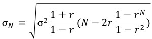
(Figure 3: Volatility Scaling with Autocorrelation Component)
So, let us estimate the volatility of the S&P 500 for different scale periods with and without taking the autocorrelation process into account. Our calculations are based on the daily logarithmic return of the 5-year time frame period from July 14th, 2017 to July 15th, 2022. The daily volatility for the analyzed period of time is 1.31% while the autocorrelation coefficient of the S&P 500 returns with lag 1 is equal to -0.20 (it is surprisingly high). It means, if the stock market decreases a lot, it is more likely to rebound on the following day, and vice versa.
| Scaling Days | Volatility Without Autocorrelation | Volatility With Autocorrelation |
| 1 | 1.31% | 1.31% |
| 5 | 2.93% | 2.50% |
| 21 | 6.01% | 4.96% |
| 252 | 20.83% | 17.03% |
In Figure 4, we can notice that the S&P 500 volatility is lower in the case of autocorrelation, which corresponds with the fact that there is a negative autocorrelation coefficient. Therefore, in terms of long-term volatility, the negative autocorrelation acts like a stabilizer. If we had positive autocorrelation, volatility estimated with the autocorrelation component would be higher than without that component. In our case, we can notice that the estimation with autocorrelation for the 1-year scaling (252 trading days) identifies that investments in the S&P 500 get a lower grade of risk than the estimation based on the assumption of stock returns independency.
Stocks Selection with IKF
While volatility enables us to estimate the risk of our investments, the I Know First AI algorithm allows us to find the most promising stocks for our investment portfolio. For example, below you can see the investment result of our World Indices package which was recommended to our clients for the period from November 24th, 2020 to July 5th, 2022 (you can access our forecast packages here).

The investment strategy that was recommended by I Know First accumulated a return of 257.79%, which exceeded the S&P 500 return by 250.87%.
Conclusion
Autocorrelation estimates the degree of similarity between a time series and a lagged version of itself, and it allows us to estimate the risk of our investment portfolio in a more precise way. We have found that the S&P 500 returns are characterized by negative autocorrelation, which means that the S&P 500 has a lower grade of risk than the estimation based on the assumption of stock returns independency. While volatility enables us to estimate the risk of our investments, the I Know First AI algorithm allows us to find the most promising stocks for our investment portfolio.

To subscribe today click here.
Please note-for trading decisions and use the most recent forecast.