
VaR Estimation: Variance-Covariance and Historical Simulation Methods
 This VaR Estimation article was written by Sergey Okun – Senior Financial Analyst at I Know First, Ph.D. in Economics.
Highlights
- VaR allows us to estimate possible financial losses in different scenarios.
- Historical Simulation VaR provides us with a result which is significantly different from respective Variance-Covariance VaR for very high confidence intervals.
- The I Know First AI algorithm provides us with the tool to select the most promising stocks.

Investors who buy assets expect to earn returns over the time horizon that they hold the asset. At the same time, actual returns over this holding period may be very different from the expected returns, and this difference between actual and expected returns is the source of risk. Volatility is the most popular measure of risk. However, volatility does not take into account the direction of a stock movement. A stock may be volatile even if it suddenly jumps higher which might not create stress for an investor. At the same time, Value at Risk (VaR) allows us to estimate possible financial losses within a portfolio over a specific time frame. It answers the questions “What is my worst-case scenario?” and “How much could I lose in a really bad day?”. VaR enables us to estimate what loss we should expect at different percentile levels.
Let us see the following two methods of VaR estimation: Variance-Covariance (VCV VaR) and Historical Simulation (HS VaR). The Historical Simulation method is based on the assumption that history repeats itself and we stick with the actual empirical distribution of return. The Variance-Covariance method is based on the assumption that there is a normal distribution for stock returns. So, let us assume for simplicity that we have the equal-weighted portfolio of the next stocks: Apple Inc. (AAPL), Amazon.com, Inc. (AMZN), Bank of America Corporation (BAC), ConocoPhillips (COP), and Pfizer Inc. (PFE).
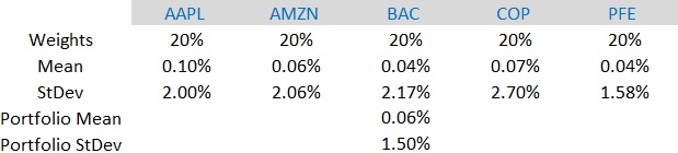

In Figures 1 and 2 we can see the statistical description of the stocks and the equal-weighted portfolio. The parameters are calculated based on the log return of daily close prices for the period from May 22, 2017, to May 23, 2022. We can notice that the daily return of the equal-weighted portfolio is 0.06% with the volatility of 1.50%.

(Figure 3: – Variance-Covariance VaR)

(Figure 4: Historical Simulation VaR)
Now according to the above equations, we can calculate VaR based on Variance-Covariance (VCV VaR) and Historical Simulation (HS VaR) techniques.

Let us assume that the value of our portfolio is $100 000. Figure 5 shows the possible losses of our portfolio according to different threshold levels. So, according to the VCV VaR, our portfolio could lose 1.87% or 3.44% of its value if one of the 10% (the confidence interval of 90%) or 1% (the confidence interval of 99% ) worse scenarios realizes. Also, we can notice that the HS VaR is significantly different from the respective VCV VaR for very high confidence intervals. For example, for the confidence interval of 99%, the HS VaR is 4.30% while VCV VaR is 3.44%. This difference is because we do not assume normality for historical simulation and we stick with the actual empirical distribution, which, in most cases of stock returns, has much fatter tails than the normal distribution has.
Stocks Selection with IKF
Value at Risk allows us to estimate possible financial losses in different scenarios. Moreover, VaR could be used as an additional constraint in the portfolio optimization task (for example, in this article we optimize a portfolio based on the four moments utility function). However, the question of the selection of promising stocks is at the discretion of investors, and it is where I Know First can help. I Know First provides different forecast packages based on the AI algorithm which allows us to select the most promising stocks (you can access them here). For example, below you can see the investment result of our S&P500 Stocks package which was recommended to our clients for the period from December 29th, 2020 to June 1st, 2022.

The investment strategy that was recommended by I Know First accumulated a return of 35.65%, which exceeded the S&P 500 return by 24.78%.
VaR Estimation: Conclusion
Value at Risk allows us to estimate possible financial losses within a portfolio over a specific time frame. It answers the questions “What is my worst-case scenario?” and “How much could I lose in a really bad day?”. In this article, we estimate VaR of a portfolio based on Variance-Covariance and Historical Simulation methods. We can notice that Historical Simulation VaR is significantly different from respective Variance-Covariance VaR for very high confidence intervals. This difference is that we do not assume normality for historical simulation and we stick with the actual empirical distribution, which, in most cases of stock returns, has much fatter tails than the normal distribution has. While VaR allows us to estimate possible financial losses in different scenarios, the I Know First AI algorithm provides us with the tool which enables us to select the most promising stocks.

To subscribe today click here.
Please note-for trading decisions and use the most recent forecast.